Testing significance of collective events with randomisation
Source:vignettes/ARCOS-randomisation.Rmd
ARCOS-randomisation.RmdIntro
This notebook demonstrates how to test the hypothesis that the statistics of collective events (CEs) differ from the statistics calculated in a random dataset.
The dataset used in this example was generated with NetLogo agent-based simulation that models collective activation events in a 2D epithelium. In the model, 2500 cells were placed on a 50x50 hexagonal grid. Collective events appear sparsely in the epithelium, they propagate radially from a source cell up to 3 cell rows. There is a 15% failure for a cell to propagate the wave, therefore the events are not always perfectly symmetrical. The simulation lasts 200 iterations.
Collective events are identified with ARCOS. To calculate the p value of a sample statistic, 5 different randomisationping methods are applied:
- shuffling entire single-cell tracks in space,
- randomly shifting entire single-cell tracks back or forth in time,
- shuffling time points independently for each track,
- shuffling the measurement between space independently for each time frame,
- shuffling activity blocks independently for each track.
Set the parameters
library(ARCOS)
library(parallel, quietly = T)
library(data.table, quietly = T)

library(ggplot2, quietly = T)
library(ggthemes, quietly = T)
library(viridis, quietly = T)

## Definitions

lPar = list()
lPar$fIn = system.file('synthetic2D/Gradient20.csv.gz',
                       package = 'ARCOS')

# Parameters for tracking collective events
lPar$db.eps = 1.5 # neighbourhood size; units of pixels
lPar$db.minPts = 3L # minimum number of cells in a cluster

lPar$trackLinkFrames = 1L # no. of subsequent frames to link during tracking; units of frames

lPar$coll.mindur = 2L # minimum duration of collective events
lPar$coll.mintotsz = lPar$db.minPts # minimum total size of collective events

lPar$debug = T

# Parameters for randomisationping
lPar$ncores = 2L # number of parallel cores
lPar$nboot = 100L # number of randomisationping iterations

# Dataset limits for plotting
lPar$limxy = c(-25, 25)
lPar$limt = c(0, 220)

# True size and duration of a single synthetic event
lPar$sim.cltotsz = 37
lPar$sim.cldur = 9

# True maximum diameter evolution of a single event in time
ttrueDiam = data.table(tevent = 0:8,
                       diam = c(2.236068, 4.472136, rep(6.708204,7)))

# Column names
lCols = list(frame = 'frame',
             posx = 'x',
             posy = 'y',
             trackid = 'id',
             meas = 'meas',
             measresc = 'meas.resc',
             measbin = 'meas.bin',
             cltrackid = 'collid',
             bootiter = 'bootiter')
Neighbourhood size for dbscan: 1.50 [px]
Minimum cluster size for dbscan: 3 [cells]
Number of subsequent frames to link: 1 [frames]
Minimum duration of collective events: 2 [frames]
Minimum total size of collective events: 3 [cells]
Number of randomisationping iterations: 100
Read data
Read a compressed CSV file, Gradient20.csv.gz from the
NetLogo simulation output. The dataset is included with the ARCOS
package. The function loadDataFromFile is a wrapper for
data.table::fread. It reads the file and sets the
attributes of the ARCOS object according to parameters defined
above.
# read data
ts = ARCOS::loadDataFromFile(lPar$fIn,
                             colPos = c(lCols$posx, lCols$posy),
                             colMeas = lCols$meas,
                             colFrame = lCols$frame,
                             colIDobj = lCols$trackid)
The dataset is in long format where each row corresponds to the measurement and position of a single object/cell at a particular point in time:
| frame | id | x | y | startCE | meas |
|---|---|---|---|---|---|
| 0 | 0 | -12 | -4.5 | 0 | 0 |
| 0 | 1 | 19 | 19.0 | 0 | 0 |
| 0 | 2 | -15 | 4.0 | 0 | 0 |
| 0 | 3 | 12 | -17.5 | 0 | 0 |
| 0 | 4 | 6 | -15.5 | 0 | 0 |
| 0 | 5 | 23 | 25.0 | 0 | 0 |
The columns have the following data:
-
frame, time frames, -
id, object/cell IDs, -
xandy, object coordinates, -
startCE, an indication of when a collective event is initiated in the simulation, -
meas, the measurement.
Identify activity
Here we identify activity pulses in single cells by using a simple
thresholding method, i.e. all measurements above 0 are considered
active. The function binMeas adds two new columns
to the dataset, meas.resc and meas.bin with
rescaled and binarised measurements, respectively.
The parameter smoothK=1 indicates that the smoothing
window initially applied to the time series is a single time point, thus
no smoothing is performed. The result of thresholding is equivalent to
calculating meas > 0.
# binarise the measurement
ARCOS::binMeas(ts,
               biasMet = "none",
               smoothK = 1,
binThr = 0.)| frame | id | x | y | startCE | meas | meas.resc | meas.bin |
|---|---|---|---|---|---|---|---|
| 0 | 0 | -12 | -4.5 | 0 | 0 | 0 | 0 |
| 1 | 0 | -12 | -4.5 | 0 | 0 | 0 | 0 |
| 2 | 0 | -12 | -4.5 | 0 | 0 | 0 | 0 |
| 3 | 0 | -12 | -4.5 | 0 | 0 | 0 | 0 |
| 4 | 0 | -12 | -4.5 | 0 | 0 | 0 | 0 |
| 5 | 0 | -12 | -4.5 | 0 | 0 | 0 | 0 |
The results of activity detection for a sample of long tracks:
ARCOS::plotBinMeas(ts,
                   ntraj = 25,
                   inSeed = 11,
                   measfac = 1.,
                   xfac = 1,
                   plotResc = F) +
  coord_cartesian(ylim = c(0,2)) +
  theme_few() +
  xlab("Time [frames]") +
  ylab("ERK activity")
#> Warning: Removed 570 rows containing missing values (`geom_path()`).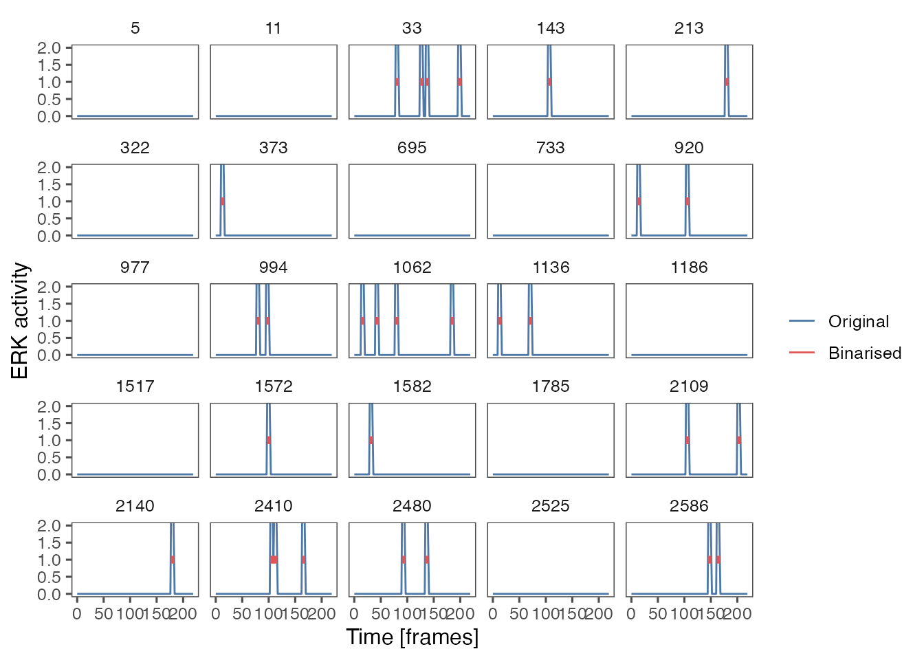
CEs - non-randomisationped
Identify collective events in the original data only for active cells, which in our case are cells with the measurement above 0.
The function trackColl returns a data table in long
format only with objects/cells that participate in collective events.
Two additional columns are added, collid.frame and
collid, with IDs of collective events per frame and a
globally unique ID, respectively. The latter, collid is
what we will use in further analysis.
# Perform tracking of collective events.
# Pass single-cell data that has a binarised measurement greater than 1.
tcoll = ARCOS::trackColl(ts[get(lCols$measbin) > 0],
                         eps = lPar$db.eps,
                         minClSz = lPar$db.minPts)

# Filter collective events based on size and duration
tcollsel = ARCOS::selColl(tcoll,
                          colldur = c(lPar$coll.mindur, Inf),
colltotsz = c(lPar$coll.mintotsz, Inf))| frame | id | collid.frame | collid | x | y | startCE | meas | meas.resc | meas.bin |
|---|---|---|---|---|---|---|---|---|---|
| 2 | 489 | 562 | 1 | 9 | 10.0 | 0 | 2 | 0.2 | 1 |
| 2 | 1150 | 562 | 1 | 10 | 8.5 | 0 | 2 | 0.2 | 1 |
| 2 | 1863 | 562 | 1 | 9 | 9.0 | 0 | 10 | 1.0 | 1 |
| 2 | 2112 | 562 | 1 | 8 | 8.5 | 0 | 2 | 0.2 | 1 |
| 2 | 2392 | 562 | 1 | 10 | 9.5 | 0 | 2 | 0.2 | 1 |
| 2 | 2427 | 562 | 1 | 8 | 9.5 | 0 | 2 | 0.2 | 1 |
Cluster properties
CE growth
Evolution of CEs’ growth quantified by the maximum Feret diameter (longer side of a minimal oriented bounding box). Red dots indicate the true evolution of a single synthetic event. Note horizontal shifts to avoid overplotting!
We observe that the majority of collective events grow as a prototypical synthetic event with only few events that depart this dynamics due to overlaps with other events.
# Calculate the minimal bounding box
tcollselDiam = calcGrowthColl(tcollsel)
The function calcGrowthColl adds the width, height and
the time of collective events’ evolution. The longer of the width and
height is taken as the diameter of the event.
| frame | collid | w | h | n | diam | tevent |
|---|---|---|---|---|---|---|
| 2 | 1 | 2.24 | 1.79 | 7 | 2.24 | 0 |
| 3 | 1 | 4.47 | 3.58 | 19 | 4.47 | 1 |
| 3 | 2 | 2.24 | 1.79 | 7 | 2.24 | 0 |
| 4 | 1 | 6.71 | 5.37 | 37 | 6.71 | 2 |
| 4 | 2 | 4.47 | 3.58 | 19 | 4.47 | 1 |
| 5 | 1 | 6.71 | 5.37 | 37 | 6.71 | 3 |
ggplot(tcollselDiam,
       aes(x = tevent,
           y = diam,
           group = get(lCols$cltrackid))) +
  geom_line(position = position_dodge(.5), alpha = 0.5) +
  geom_point(data = ttrueDiam,
             aes(x = tevent,
                 y = diam,
                 group = 1),
             colour = 'red') +
  xlab("Time [frames]") +
  ylab('Diameter [au]') +
  theme_minimal()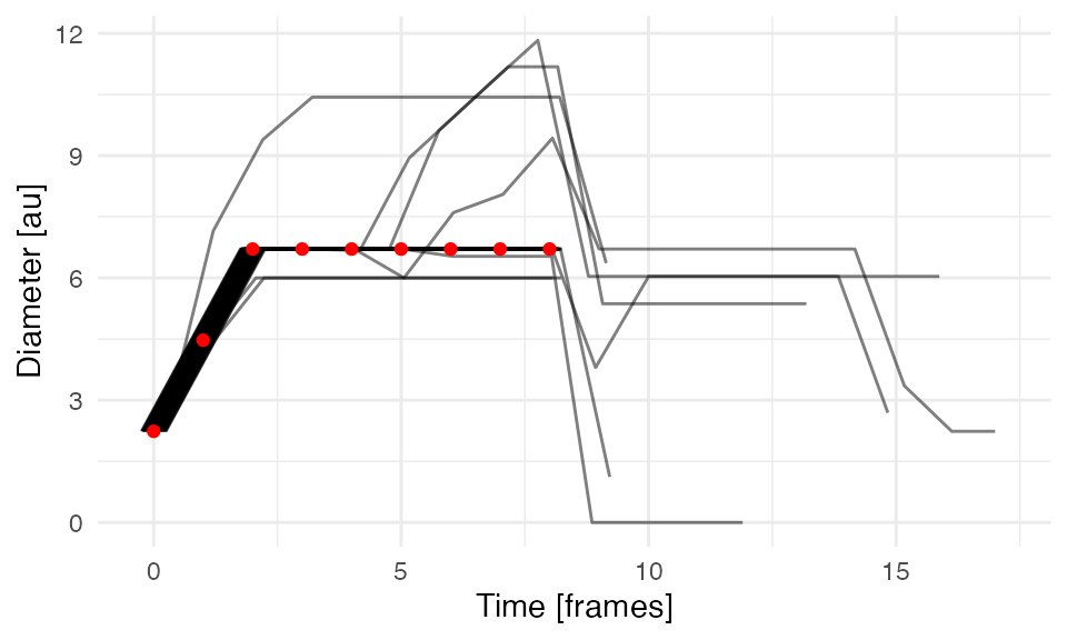
Duration & total size
We extract two statistics of collective events: event duration and the total number of unique cells involved in an event (~ size). Dashed lines indicate true size & duration of synthetic events. Several bigger and longer-lasting than synthetic events are due to overlap with other events.
# Calculate duration of collective events in frames
tcollselAggr = ARCOS::calcStatsColl(tcollsel)


ggplot(tcollselAggr,
       aes(x = totSz,
           y = clDur)) +
  geom_hex() +
  viridis::scale_fill_viridis(discrete = F,
                              trans = "log10") +
  geom_vline(xintercept = lPar$sim.cltotsz, color = "red", linetype = 2) +
  geom_hline(yintercept = lPar$sim.cldur, color = "red", linetype = 2) +
  xlab("#cells involved in collective events") +
  ylab("Duration of collective events [#frames]") +
  theme_bw()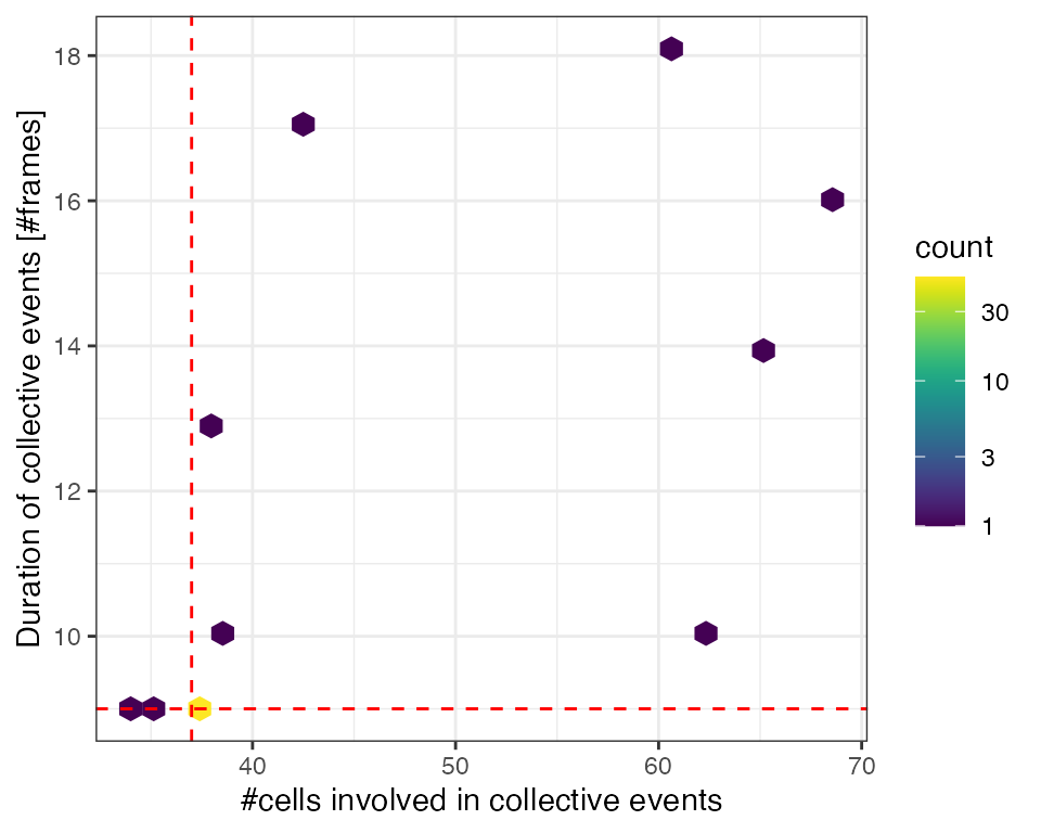
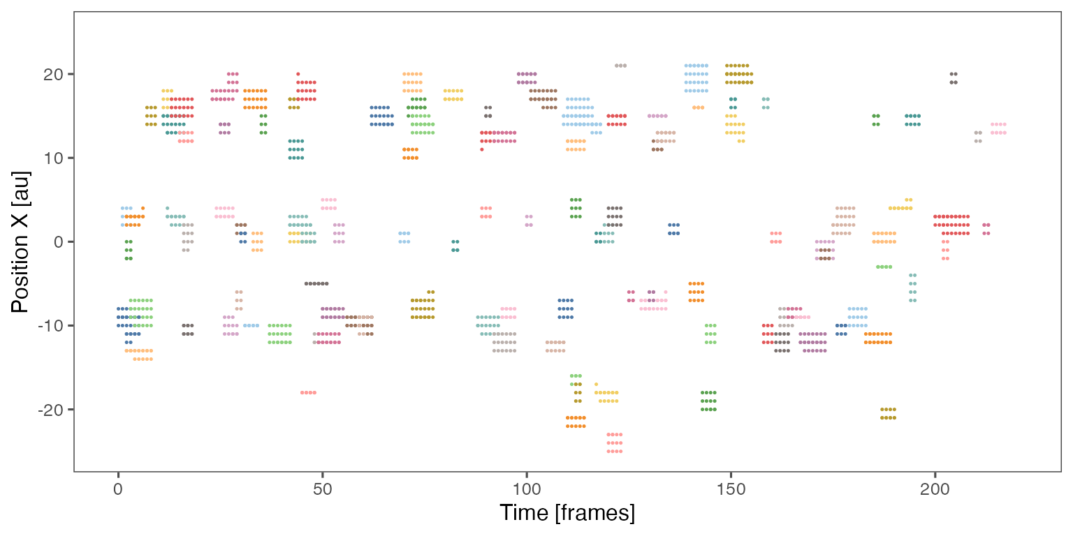
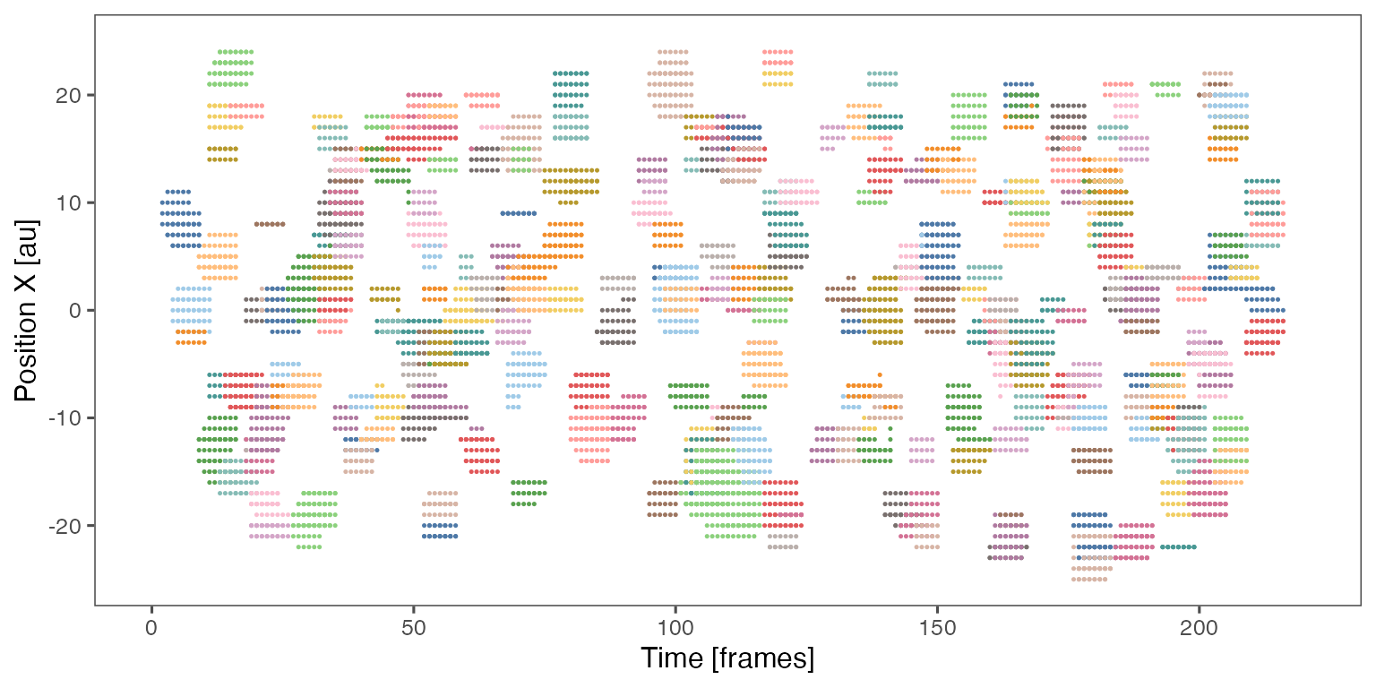
Noodle plot
X/T projection of individual cells that participate in collective events. Tracks are coloured by the IS of collective events. Red dots indicate the beginning of a spontaneous collective event in the simulation.
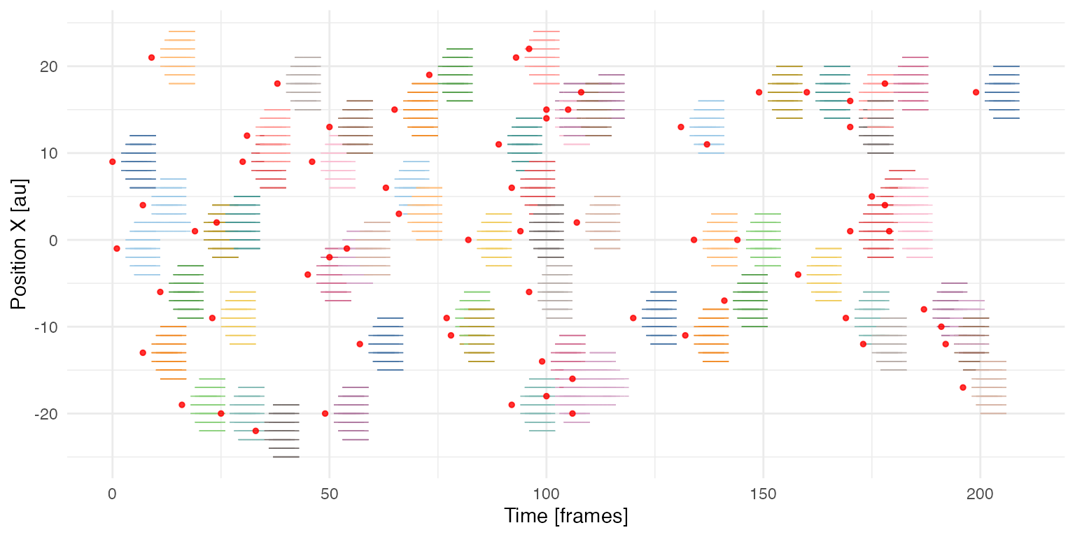
Number of initiated events: 69
Number of detected events: 61
Average binarised activity level: 0.0294
Fraction of activity in (filtered) collective events: 0.9957
CEs - randomisationed
Calculate p-values for the two statistics (duration and size) using randomisationping. Each calculation can take up to several minutes!
Shuffle initial XY
In this approach, the initial position of every track is shuffled between all cells in the system. Since the measurement dynamics remains intact, this approach randomises only the spatial aspect of collective phenomena, i.e. tracks are only rearranged in space while retaining their measurement dynamics. One caveat concerns cases where cells/objects are moving in space. By assigning new starting points, objects’ positions may exceed the initial bounds of the field of view.
The ARCOS::trackCollBoot function outputs a
data.table in long format with time points when individual
objects participate in collective events. From this output, further
statistics can be extracted, such as: duration, size, diameter, number
of collective events. The bootiter column indexes
randomisationping iterations.
# Perform randomisation or load data from a file
stmp = system.file(sprintf('synthetic2D/output-randomisation-20/randRes_shuffIniXY_N%d.csv.gz', lPar$nboot),
                   package = 'ARCOS')

if (file.exists(stmp)) {

  tcollselBoot = ARCOS::loadDataFromFile(fname = stmp,
                                         colPos = c(lCols$posx, lCols$posy),
                                         colFrame = lCols$frame,
                                         colIDobj = lCols$trackid,
                                         colIDcoll = lCols$cltrackid,
                                         colBootIter = lCols$bootiter,
                                         fromColl = TRUE,
                                         fromBoot = TRUE)
} else {
  set.seed(11)

  tcollselBoot = ARCOS::trackCollBoot(obj = ts,
                                      nboot = lPar$nboot,
                                      ncores = lPar$ncores,
                                      method = 'shuffCoord',
                                      eps = lPar$db.eps,
                                      epsPrev = lPar$db.eps,
                                      nPrev = 1L,
                                      minClSz = lPar$db.minPts,
                                      colldurlim = c(lPar$coll.mindur, 1000),
                                      colltotszlim = c(lPar$coll.mintotsz, 1000),
                                      deb = F)

  #fwrite(tcollselBoot, file = sprintf('../inst/synthetic2D/output-randomisation-20/bootRes_shuffIniXY_N%d.csv.gz', lPar$nboot))
}| bootiter | frame | id | collid.frame | collid | x | y | startCE | meas | meas.resc | meas.bin | meas.bin.shuff |
|---|---|---|---|---|---|---|---|---|---|---|---|
| 1 | 11 | 120 | 130 | 1 | -19 | -11.0 | 0 | 2 | 0.2 | 1 | 1 |
| 1 | 11 | 145 | 130 | 1 | -18 | -9.5 | 0 | 2 | 0.2 | 1 | 1 |
| 1 | 11 | 186 | 129 | 2 | -18 | -13.5 | 0 | 10 | 1.0 | 1 | 1 |
| 1 | 11 | 288 | 130 | 1 | -18 | -10.5 | 0 | 8 | 0.8 | 1 | 1 |
| 1 | 11 | 723 | 130 | 1 | -17 | -11.0 | 0 | 2 | 0.2 | 1 | 1 |
| 1 | 11 | 1734 | 129 | 2 | -19 | -13.0 | 0 | 2 | 0.2 | 1 | 1 |
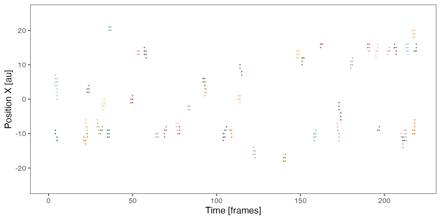
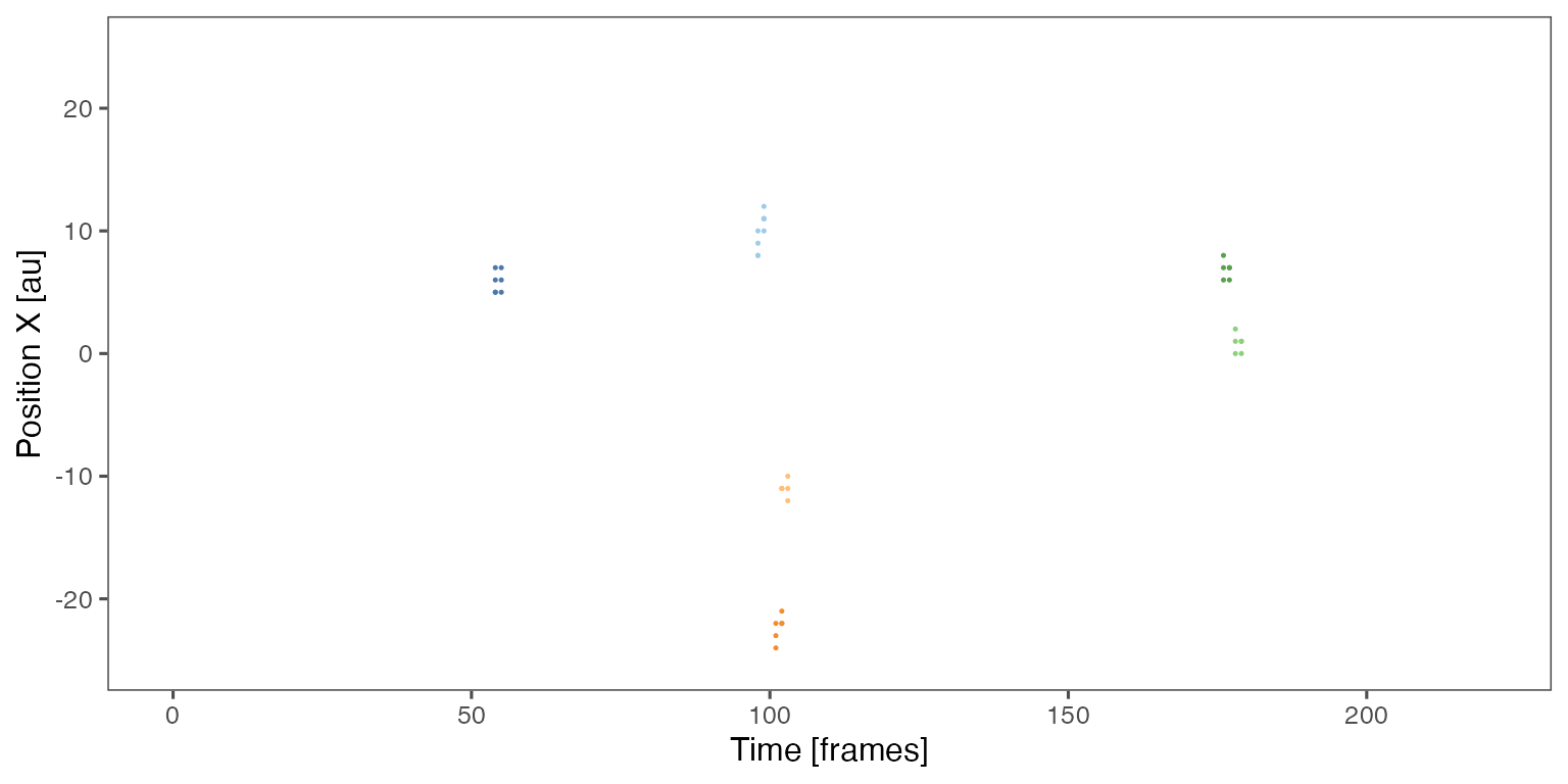
Sample noodle plot from a single randomisation iteration:
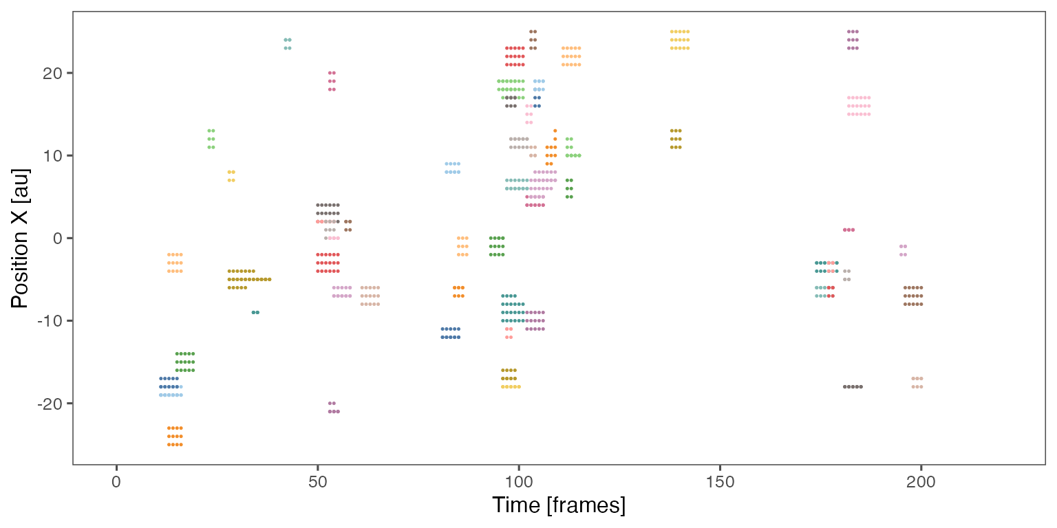
Distribution of the fraction of collective events in randomisation iterations compared to the observed fraction (red dashed line):
tFracActInColl = calcFracActInColl(ts, tcollsel)
tFracActInCollBoot = calcFracActInColl(ts, tcollselBoot)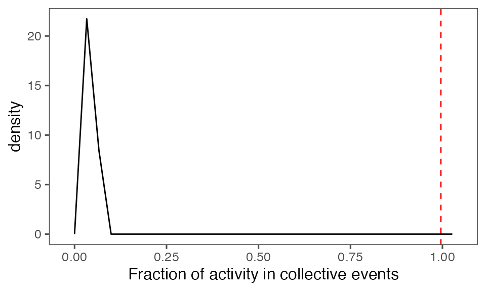
P-value, alternative hypothesis - the fraction of total (binarised) activity involved in observed collective events is greater than the mean fraction in randomised events:
calcPvalFromBS(tFracActInColl, tFracActInCollBoot$fracAct, corrected = T, alternative = 'greater')
#> [1] 0.00990099
Aggregate statistics from iterations:
# Aggregate the results of randomisationping per collective event
tcollbootAggrPerColl = calcStatsColl(tcollselBoot)
# Further aggregate size & duration per randomisation iteration
tcollbootSzDurPerIter = tcollbootAggrPerColl[,
lapply(.SD, mean),
by = c(lCols$bootiter),
.SDcols = c('clDur', 'totSz', 'minSz', 'maxSz')]
# Further aggregate the number of events per randomisation iteration
tcollbootNcollPerIter = tcollbootAggrPerColl[,
.(N = sum(!is.na(get(lCols$cltrackid)))),
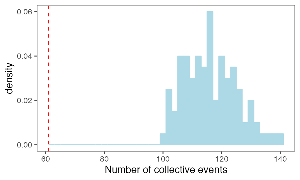
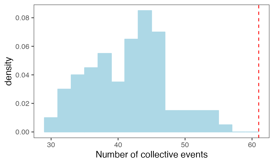
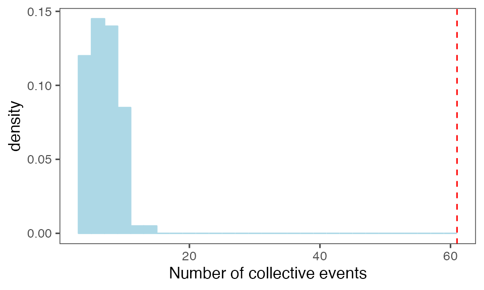
by = c(lCols$bootiter)]Distribution of the number of collective events identified in every randomisation iteration compared to the observed statistics (red dashed line):
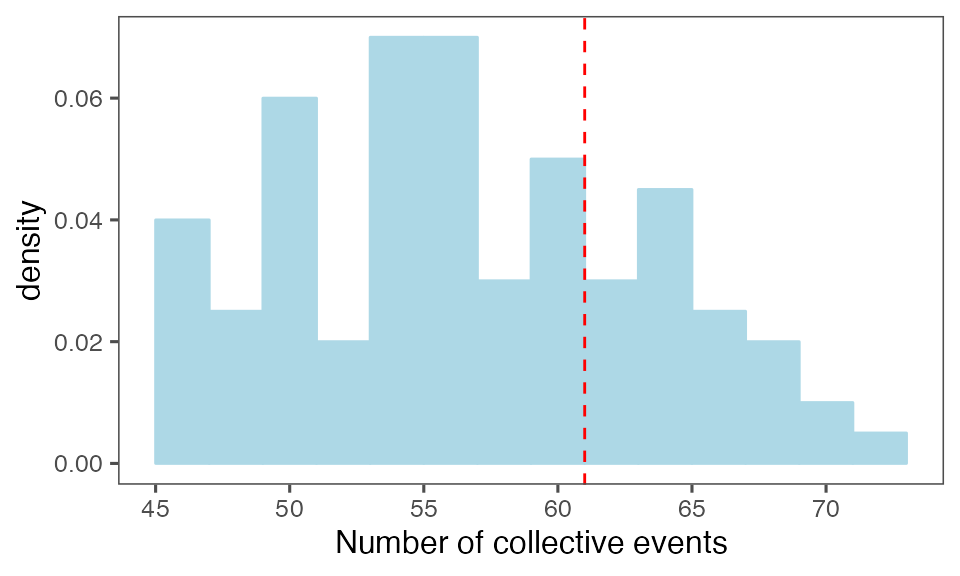
P-value, alternative hypothesis - the number of observed CEs is less than the mean number of clusters in randomised data:
calcPvalFromBS(nrow(tcollselAggr), tcollbootNcollPerIter$N, corrected = T, alternative = 'less')
#> [1] 0.7326733
P-value, alternative hypothesis - the number of observed CEs is greater than the mean number of clusters in randomised data:
calcPvalFromBS(nrow(tcollselAggr), tcollbootNcollPerIter$N, corrected = T, alternative = 'greater')
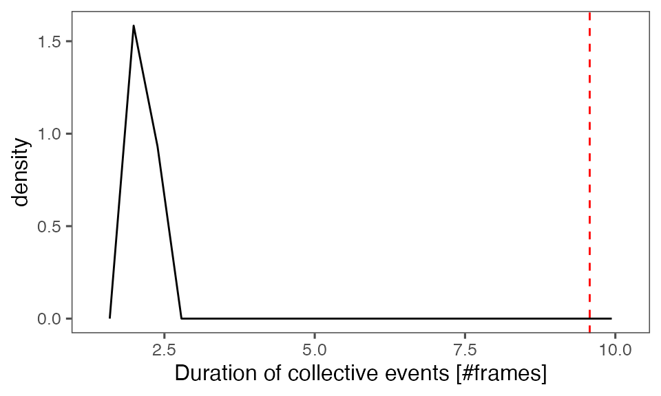
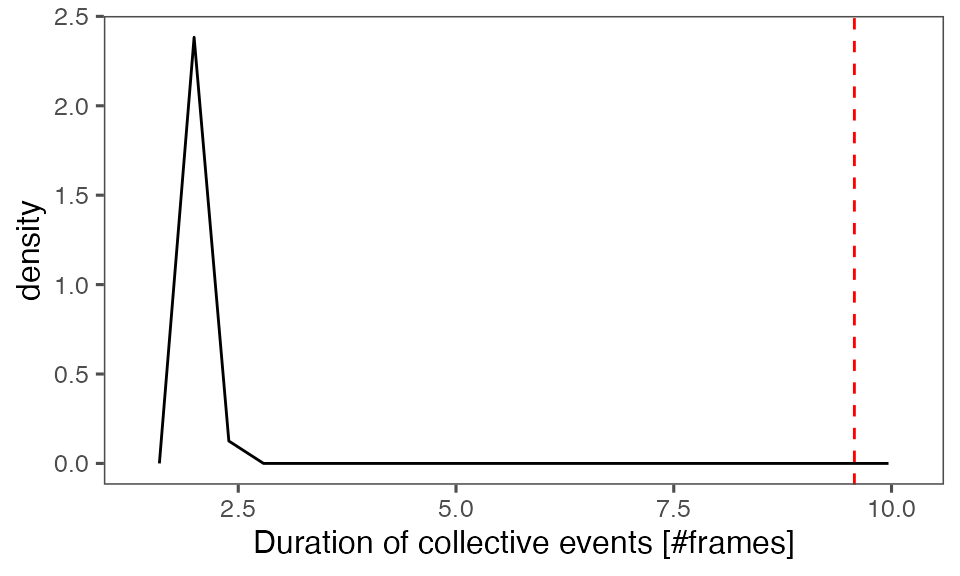
#> [1] 0.3168317Distribution of the mean cluster duration from randomisation iterations (solid black line) vs. the mean cluster duration from the non-randomised data (red dashed line):
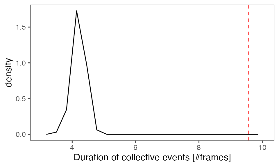
P-value, alternative hypothesis - the mean observed cluster duration is greater than the mean cluster duration in randomised data:
calcPvalFromBS(mean(tcollselAggr$clDur), tcollbootSzDurPerIter$clDur, corrected = T, alternative = 'greater')
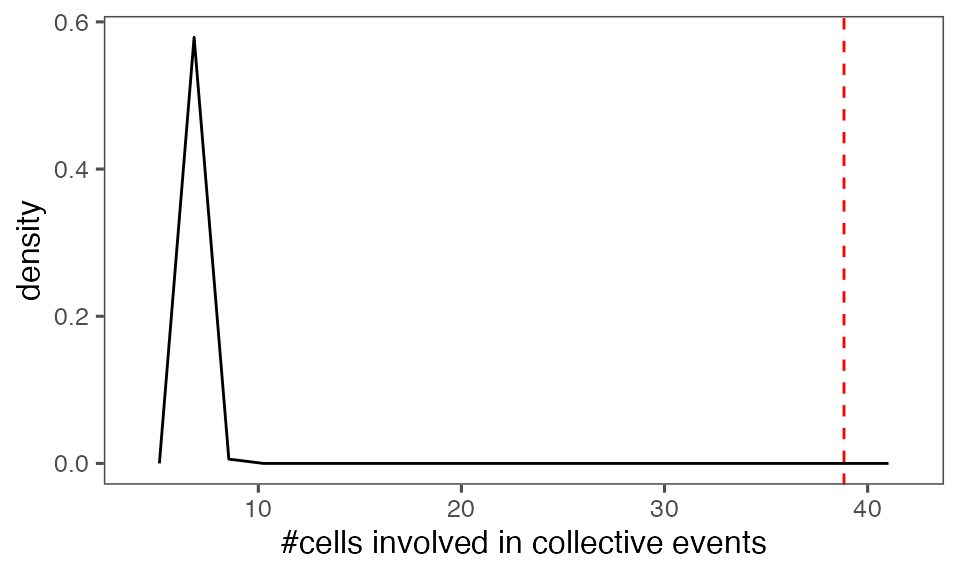
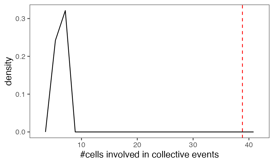
#> [1] 0.00990099Distribution of the mean total cluster size from randomisation iterations (solid black line) vs. the mean total cluster size from the non-randomised data (red dashed line):
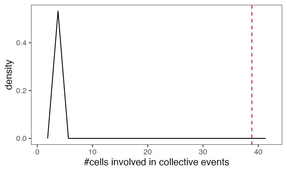
P-value, alternative hypothesis - the mean observed total cluster size is greater than the cluster size in randomised data:
calcPvalFromBS(mean(tcollselAggr$totSz), tcollbootSzDurPerIter$totSz, corrected = T, alternative = 'greater')
#> [1] 0.00990099
Randomly shift the measurement
Here, entire single-cell tracks are shifted forward or backward in time. The spatial arrangement of cells and the measurement dynamics are intact, except activation events occur at different times than originally.
stmp = system.file(sprintf('synthetic2D/output-randomisation-20/randRes_randShiftMeas_N%d.csv.gz', lPar$nboot),
                   package = 'ARCOS')

if (file.exists(stmp)) {
  tcollselBoot = loadDataFromFile(fname = stmp,
                                  colPos = c(lCols$posx, lCols$posy),
                                  colFrame = lCols$frame,
                                  colIDobj = lCols$trackid,
                                  colIDcoll = lCols$cltrackid,
                                  colMeas = lCols$meas,
                                  colBootIter = lCols$bootiter,
                                  fromColl = TRUE,
                                  fromBoot = TRUE)
} else {
  set.seed(11)

  tcollselBoot = ARCOS::trackCollBoot(obj = ts,
                                      nboot = lPar$nboot,
                                      ncores = lPar$ncores,
                                      method = 'randShiftMeas',
                                      eps = lPar$db.eps,
                                      epsPrev = lPar$db.eps,
                                      nPrev = 1L,
                                      minClSz = lPar$db.minPts,
                                      colldurlim = c(lPar$coll.mindur, 1000),
                                      colltotszlim = c(lPar$coll.mintotsz, 1000),
                                      deb = F)

  #fwrite(tcollselBoot, file = sprintf('../inst/synthetic2D/output-randomisation-20/bootRes_randShiftMeas_N%d.csv.gz', lPar$nboot))
}| bootiter | frame | id | collid.frame | collid | x | y | startCE | meas | meas.resc | meas.bin | meas.bin.shuff |
|---|---|---|---|---|---|---|---|---|---|---|---|
| 1 | 0 | 33 | 87 | 1 | -9 | -19.0 | 0 | 0 | 0 | 0 | 1 |
| 1 | 0 | 112 | 87 | 1 | -8 | -19.5 | 0 | 0 | 0 | 0 | 1 |
| 1 | 0 | 760 | 87 | 1 | -10 | -18.5 | 0 | 0 | 0 | 0 | 1 |
| 1 | 0 | 2148 | 87 | 1 | -9 | -18.0 | 0 | 0 | 0 | 0 | 1 |
| 1 | 1 | 33 | 88 | 1 | -9 | -19.0 | 0 | 0 | 0 | 0 | 1 |
| 1 | 1 | 112 | 88 | 1 | -8 | -19.5 | 0 | 0 | 0 | 0 | 1 |
Sample noodle plot from a single randomisation iteration:
Distribution of the fraction of collective events in randomisation iterations compared to the observed fraction (red dashed line):
tFracActInColl = calcFracActInColl(ts, tcollsel)
tFracActInCollBoot = calcFracActInColl(ts, tcollselBoot)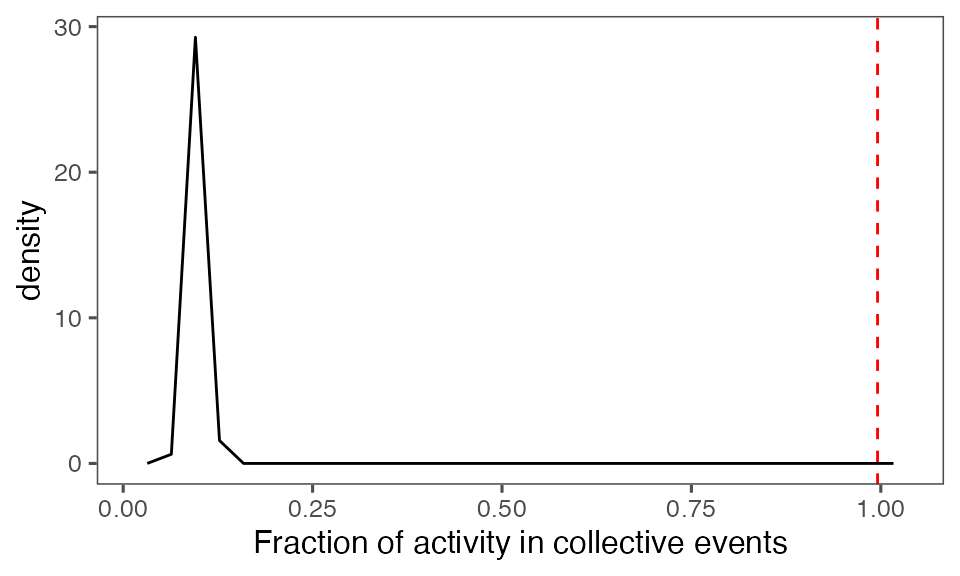
P-value, alternative hypothesis - the fraction of total (binarised) activity involved in observed collective events is greater than the mean fraction in randomised events:
calcPvalFromBS(tFracActInColl, tFracActInCollBoot$fracAct, corrected = T, alternative = 'greater')
#> [1] 0.00990099
Aggregate statistics from iterations:
# Aggregate the results of randomisationping per collective event
tcollbootAggrPerColl = calcStatsColl(tcollselBoot)

# Further aggregate size & duration per randomisation iteration
tcollbootSzDurPerIter = tcollbootAggrPerColl[,
                                             lapply(.SD, mean),
                                             by = c(lCols$bootiter),
                                             .SDcols = c('clDur', 'totSz', 'minSz', 'maxSz')]

# Further aggregate the number of events per randomisation iteration
tcollbootNcollPerIter = tcollbootAggrPerColl[,
                                             .(N = sum(!is.na(get(lCols$cltrackid)))),
                                             by = c(lCols$bootiter)]
Distribution of the number of collective events identified in every randomisation iteration compared to the observed statistics (red dashed line):
P-value, alternative hypothesis - the number of observed CEs is less than the mean number of clusters in randomised data:
calcPvalFromBS(nrow(tcollselAggr), tcollbootNcollPerIter$N, corrected = T, alternative = 'less')
#> [1] 0.00990099
Distribution of the mean cluster duration from randomisation iterations (solid black line) vs. the mean cluster duration from the non-randomised data (red dashed line):

P-value, alternative hypothesis - the mean observed cluster duration is greater than the mean cluster duration in randomised data:
calcPvalFromBS(mean(tcollselAggr$clDur), tcollbootSzDurPerIter$clDur, corrected = T, alternative = 'greater')
#> [1] 0.00990099
Distribution of the mean total cluster size from randomisation iterations (solid black line) vs. the mean total cluster size from the non-randomised data (red dashed line):

P-value, alternative hypothesis - the mean observed total cluster size is greater than the cluster size in randomised data:
calcPvalFromBS(mean(tcollselAggr$totSz), tcollbootSzDurPerIter$totSz, corrected = T, alternative = 'greater')
#> [1] 0.00990099
Shuffle time points per track
Here, individual time points are shuffled independently in each track. While the spatial arrangement is intact, the measurement dynamics is completely randomised.
stmp = system.file(sprintf('synthetic2D/output-randomisation-20/randRes_shuffMeasTrack_N%d.csv.gz', lPar$nboot),
                   package = 'ARCOS')

if (file.exists(stmp)) {
  tcollselBoot = loadDataFromFile(fname = stmp,
                                  colPos = c(lCols$posx, lCols$posy),
                                  colFrame = lCols$frame,
                                  colIDobj = lCols$trackid,
                                  colIDcoll = lCols$cltrackid,
                                  colMeas = lCols$meas,
                                  colBootIter = lCols$bootiter,
                                  fromColl = TRUE,
                                  fromBoot = TRUE)
} else {
  set.seed(11)

  tcollselBoot = ARCOS::trackCollBoot(obj = ts,
                                      nboot = lPar$nboot,
                                      ncores = lPar$ncores,
                                      method = 'shuffMeasTrack',
                                      eps = lPar$db.eps,
                                      epsPrev = lPar$db.eps,
                                      nPrev = 1L,
                                      minClSz = lPar$db.minPts,
                                      colldurlim = c(lPar$coll.mindur, 1000),
                                      colltotszlim = c(lPar$coll.mintotsz, 1000),
                                      deb = F)

  #fwrite(tcollselBoot, file = sprintf('../inst/synthetic2D/output-randomisation-20/bootRes_shuffMeasTrack_N%d.csv.gz', lPar$nboot))
}| bootiter | frame | id | collid.frame | collid | x | y | startCE | meas | meas.resc | meas.bin | meas.bin.shuff |
|---|---|---|---|---|---|---|---|---|---|---|---|
| 1 | 4 | 177 | 196 | 8 | -9 | -16.0 | 0 | 0 | 0 | 0 | 1 |
| 1 | 4 | 759 | 196 | 8 | -10 | -16.5 | 0 | 0 | 0 | 0 | 1 |
| 1 | 4 | 888 | 196 | 8 | -9 | -15.0 | 0 | 0 | 0 | 0 | 1 |
| 1 | 4 | 1055 | 199 | 12 | 6 | -11.5 | 0 | 0 | 0 | 0 | 1 |
| 1 | 4 | 1467 | 199 | 12 | 4 | -10.5 | 0 | 0 | 0 | 0 | 1 |
| 1 | 4 | 1569 | 199 | 12 | 6 | -10.5 | 0 | 0 | 0 | 0 | 1 |
Sample noodle plot from a single randomisation iteration:
Distribution of the fraction of collective events in randomisation iterations compared to the observed fraction (red dashed line):
tFracActInColl = calcFracActInColl(ts, tcollsel)
tFracActInCollBoot = calcFracActInColl(ts, tcollselBoot)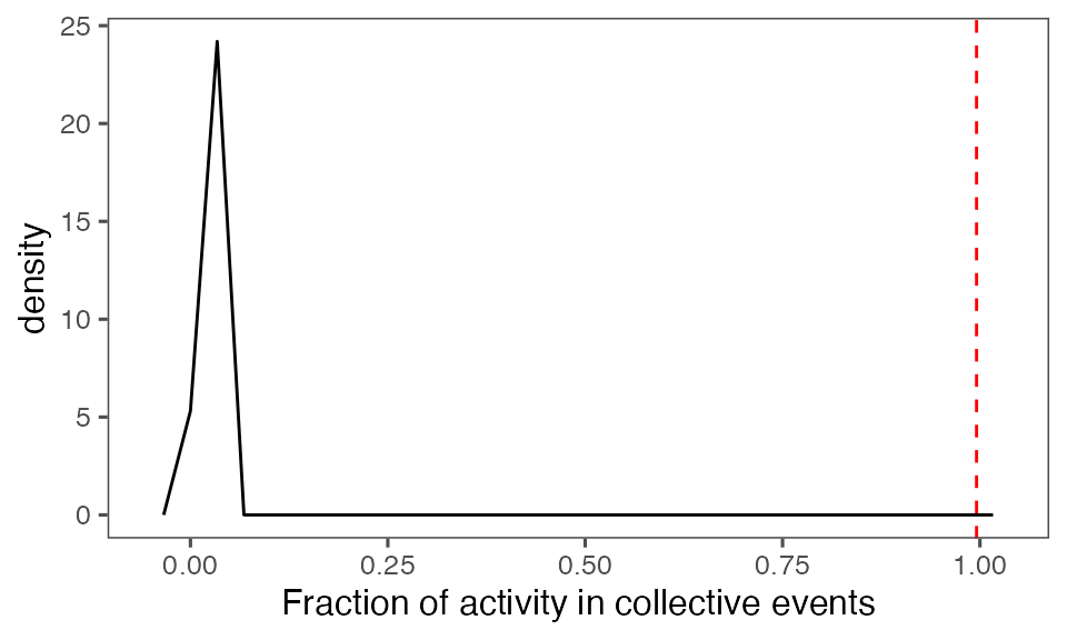
P-value, alternative hypothesis - the fraction of total (binarised) activity involved in observed collective events is greater than the mean fraction in randomised events:
calcPvalFromBS(tFracActInColl, tFracActInCollBoot$fracAct, corrected = T, alternative = 'greater')
#> [1] 0.00990099
Aggregate statistics from iterations:
# Aggregate the results of randomisationping per collective event
tcollbootAggrPerColl = calcStatsColl(tcollselBoot)

# Further aggregate size & duration per randomisation iteration
tcollbootSzDurPerIter = tcollbootAggrPerColl[,
                                             lapply(.SD, mean),
                                             by = c(lCols$bootiter),
                                             .SDcols = c('clDur', 'totSz', 'minSz', 'maxSz')]

# Further aggregate the number of events per randomisation iteration
tcollbootNcollPerIter = tcollbootAggrPerColl[,
                                             .(N = sum(!is.na(get(lCols$cltrackid)))),
                                             by = c(lCols$bootiter)]
Distribution of the number of collective events identified in every randomisation iteration compared to the observed statistics (red dashed line):
P-value, alternative hypothesis - the number of observed CEs is greater than the mean number of clusters in randomised data:
calcPvalFromBS(nrow(tcollselAggr), tcollbootNcollPerIter$N, corrected = T, alternative = 'greater')
#> [1] 0.00990099
Distribution of the mean cluster duration from randomisation iterations (solid black line) vs. the mean cluster duration from the non-randomised data (red dashed line):
P-value, alternative hypothesis - the mean observed cluster duration is greater than the mean cluster duration in randomised data:
calcPvalFromBS(mean(tcollselAggr$clDur), tcollbootSzDurPerIter$clDur, corrected = T, alternative = 'greater')
#> [1] 0.00990099
Distribution of the mean total cluster size from randomisation iterations (solid black line) vs. the mean total cluster size from the non-randomised data (red dashed line):
P-value, alternative hypothesis - the mean observed total cluster size is greater than the cluster size in randomised data:
calcPvalFromBS(mean(tcollselAggr$totSz), tcollbootSzDurPerIter$totSz, corrected = T, alternative = 'greater')
#> [1] 0.00990099
Shuffle measurement per frame
Here, binarised measurements are shuffled between cells independently in every time frame. Positions remain intact; the total activity per track is affected.
stmp = system.file(sprintf('synthetic2D/output-randomisation-20/randRes_shuffMeasFrame_N%d.csv.gz', lPar$nboot),
                   package = 'ARCOS')


if (file.exists(stmp)) {
  tcollselBoot = loadDataFromFile(fname = stmp,
                                  colPos = c(lCols$posx, lCols$posy),
                                  colFrame = lCols$frame,
                                  colIDobj = lCols$trackid,
                                  colIDcoll = lCols$cltrackid,
                                  colMeas = lCols$meas,
                                  colBootIter = lCols$bootiter,
                                  fromColl = TRUE,
                                  fromBoot = TRUE)
} else {
  set.seed(11)

  tcollselBoot = ARCOS::trackCollBoot(obj = ts,
                                      nboot = lPar$nboot,
                                      ncores = lPar$ncores,
                                      method = 'shuffMeasFrame',
                                      eps = lPar$db.eps,
                                      epsPrev = lPar$db.eps,
                                      nPrev = 1L,
                                      minClSz = lPar$db.minPts,
                                      colldurlim = c(lPar$coll.mindur, 1000),
                                      colltotszlim = c(lPar$coll.mintotsz, 1000),
                                      deb = F)

  #fwrite(tcollselBoot, file = sprintf('../inst/synthetic2D/output-randomisation-20/bootRes_shuffMeasFrame_N%d.csv.gz', lPar$nboot))
}| bootiter | frame | id | collid.frame | collid | x | y | startCE | meas | meas.resc | meas.bin | meas.bin.shuff |
|---|---|---|---|---|---|---|---|---|---|---|---|
| 1 | 54 | 4 | 13 | 44 | 6 | -15.5 | 0 | 0 | 0.0 | 0 | 1 |
| 1 | 54 | 108 | 13 | 44 | 7 | -16.0 | 0 | 0 | 0.0 | 0 | 1 |
| 1 | 54 | 675 | 13 | 44 | 5 | -15.0 | 0 | 0 | 0.0 | 0 | 1 |
| 1 | 54 | 1500 | 13 | 44 | 5 | -16.0 | 0 | 0 | 0.0 | 0 | 1 |
| 1 | 55 | 1500 | 156 | 44 | 5 | -16.0 | 0 | 0 | 0.0 | 0 | 1 |
| 1 | 55 | 1683 | 156 | 44 | 7 | -17.0 | 0 | 2 | 0.2 | 1 | 1 |
Sample noodle plot from a single randomisation iteration:
Distribution of the fraction of collective events in randomisation iterations compared to the observed fraction (red dashed line):
tFracActInColl = calcFracActInColl(ts, tcollsel)
tFracActInCollBoot = calcFracActInColl(ts, tcollselBoot)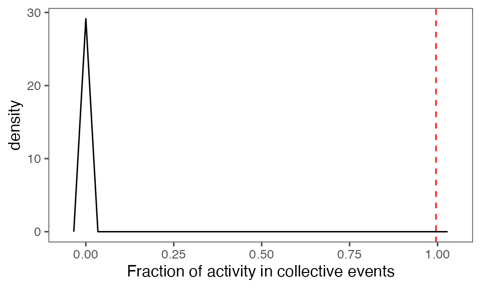
P-value, alternative hypothesis - the fraction of total (binarised) activity involved in observed collective events is greater than the mean fraction in randomised events:
calcPvalFromBS(tFracActInColl, tFracActInCollBoot$fracAct, corrected = T, alternative = 'greater')
#> [1] 0.00990099
Aggregate statistics from iterations:
# Aggregate the results of randomisationping per collective event
tcollbootAggrPerColl = calcStatsColl(tcollselBoot)

# Further aggregate size & duration per randomisation iteration
tcollbootSzDurPerIter = tcollbootAggrPerColl[,
                                             lapply(.SD, mean),
                                             by = c(lCols$bootiter),
                                             .SDcols = c('clDur', 'totSz', 'minSz', 'maxSz')]

# Further aggregate the number of events per randomisation iteration
tcollbootNcollPerIter = tcollbootAggrPerColl[,
                                             .(N = sum(!is.na(get(lCols$cltrackid)))),
                                             by = c(lCols$bootiter)]
Distribution of the number of collective events identified in every randomisation iteration compared to the observed statistics (red dashed line):
P-value, alternative hypothesis - the number of observed CEs is greater than the mean number of clusters in randomised data:
calcPvalFromBS(nrow(tcollselAggr), tcollbootNcollPerIter$N, corrected = T, alternative = 'greater')
#> [1] 0.00990099
Distribution of the mean cluster duration from randomisation iterations (solid black line) vs. the mean cluster duration from the non-randomised data (red dashed line):
P-value, alternative hypothesis - the mean observed cluster duration is greater than the mean cluster duration in randomised data:
calcPvalFromBS(mean(tcollselAggr$clDur), tcollbootSzDurPerIter$clDur, corrected = T, alternative = 'greater')
#> [1] 0.00990099
Distribution of the mean total cluster size from randomisation iterations (solid black line) vs. the mean total cluster size from the non-randomised data (red dashed line):
P-value, alternative hypothesis - the mean observed total cluster size is greater than the cluster size in randomised data:
calcPvalFromBS(mean(tcollselAggr$totSz), tcollbootSzDurPerIter$totSz, corrected = T, alternative = 'greater')
#> [1] 0.00990099
Shuffle blocks per track
In this approach, blocks of activity in binarised time series are shuffled independently in every track. Positions remain intact and the alternating order of 0 and 1 blocks is maintained.
lPar$nboot = 100
stmp = system.file(sprintf('synthetic2D/output-randomisation-20/randRes_shuffBlockTrackAlt_N%d.csv.gz', lPar$nboot),
                   package = 'ARCOS')


if (file.exists(stmp)) {
  tcollselBoot = loadDataFromFile(fname = stmp,
                                  colPos = c(lCols$posx, lCols$posy),
                                  colFrame = lCols$frame,
                                  colIDobj = lCols$trackid,
                                  colIDcoll = lCols$cltrackid,
                                  colMeas = lCols$meas,
                                  colBootIter = lCols$bootiter,
                                  fromColl = TRUE,
                                  fromBoot = TRUE)
} else {
  set.seed(11)

  tcollselBoot = ARCOS::trackCollBoot(obj = ts,
                                      nboot = lPar$nboot,
                                      ncores = lPar$ncores,
                                      method = 'shuffBlockTrackAlt',
                                      eps = lPar$db.eps,
                                      epsPrev = lPar$db.eps,
                                      nPrev = 1L,
                                      minClSz = lPar$db.minPts,
                                      colldurlim = c(lPar$coll.mindur, 1000),
                                      colltotszlim = c(lPar$coll.mintotsz, 1000),
                                      deb = F)

  #fwrite(tcollselBoot, file = sprintf('../inst/synthetic2D/output-randomisation-20/bootRes_shuffBlockTrack_N$d.csv.gz', lPar$nboot))

}| bootiter | frame | id | collid.frame | collid | x | y | startCE | meas | meas.resc | meas.bin | meas.bin.shuff |
|---|---|---|---|---|---|---|---|---|---|---|---|
| 1 | 2 | 1150 | 1749 | 1 | 10 | 8.5 | 0 | 2 | 1 | 1 | 1 |
| 1 | 2 | 1863 | 1749 | 1 | 9 | 9.0 | 0 | 10 | 1 | 1 | 1 |
| 1 | 2 | 2112 | 1749 | 1 | 8 | 8.5 | 0 | 2 | 1 | 1 | 1 |
| 1 | 3 | 805 | 1748 | 1 | 9 | 7.0 | 0 | 2 | 1 | 1 | 1 |
| 1 | 3 | 915 | 1748 | 1 | 7 | 9.0 | 0 | 2 | 1 | 1 | 1 |
| 1 | 3 | 1150 | 1748 | 1 | 10 | 8.5 | 0 | 10 | 1 | 1 | 1 |
Sample noodle plot from a single randomisation iteration:
Distribution of the fraction of collective events in randomisation iterations compared to the observed fraction (red dashed line):
tFracActInColl = calcFracActInColl(ts, tcollsel)
tFracActInCollBoot = calcFracActInColl(ts, tcollselBoot)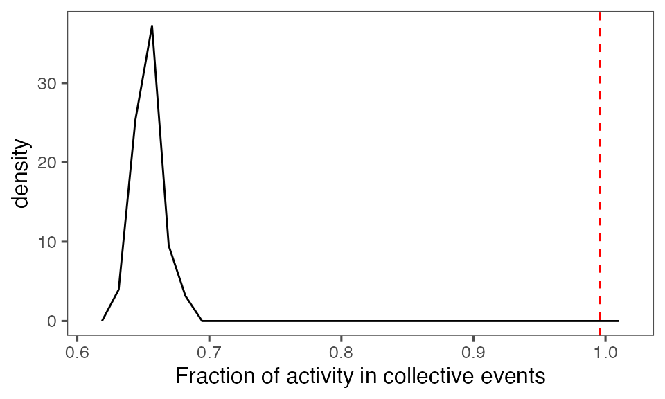
P-value, alternative hypothesis - the fraction of total (binarised) activity involved in observed collective events is greater than the mean fraction in randomised events:
calcPvalFromBS(tFracActInColl, tFracActInCollBoot$fracAct, corrected = T, alternative = 'greater')
#> [1] 0.00990099
Aggregate statistics from iterations:
# Aggregate the results of randomisationping per collective event
tcollbootAggrPerColl = calcStatsColl(tcollselBoot)

# Further aggregate size & duration per randomisation iteration
tcollbootSzDurPerIter = tcollbootAggrPerColl[,
                                             lapply(.SD, mean),
                                             by = c(lCols$bootiter),
                                             .SDcols = c('clDur', 'totSz', 'minSz', 'maxSz')]

# Further aggregate the number of events per randomisation iteration
tcollbootNcollPerIter = tcollbootAggrPerColl[,
                                             .(N = sum(!is.na(get(lCols$cltrackid)))),
                                             by = c(lCols$bootiter)]
Distribution of the number of collective events identified in every randomisation iteration compared to the observed statistics (red dashed line):
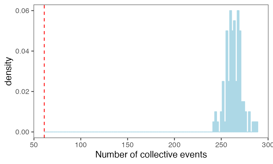
P-value, alternative hypothesis - the number of observed CEs is less than the mean number of clusters in randomised data:
calcPvalFromBS(nrow(tcollselAggr), tcollbootNcollPerIter$N, corrected = T, alternative = 'less')
#> [1] 0.00990099
Distribution of the mean cluster duration from randomisation iterations (solid black line) vs. the mean cluster duration from the non-randomised data (red dashed line):
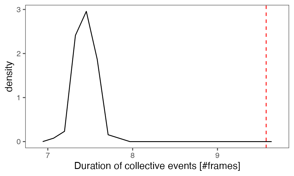
P-value, alternative hypothesis - the mean observed cluster duration is greater than the mean cluster duration in randomised data:
calcPvalFromBS(mean(tcollselAggr$clDur), tcollbootSzDurPerIter$clDur, corrected = T, alternative = 'greater')
#> [1] 0.00990099
Distribution of the mean total cluster size from randomisation iterations (solid black line) vs. the mean total cluster size from the non-randomised data (red dashed line):

P-value, alternative hypothesis - the mean observed total cluster size is greater than the cluster size in randomised data:
calcPvalFromBS(mean(tcollselAggr$totSz), tcollbootSzDurPerIter$totSz, corrected = T, alternative = 'greater')
#> [1] 0.00990099