Basic usage of ARCOS • ARCOS

library(data.table)
library(ARCOS)
library(ggplot2)
library(ggnewscale)

Intro

Automated Recognition of Collective Signalling (ARCOS) is an R package to identify collective spatial events in time series data. The associated publication is available on bioRxiv.

The software identifies and visualises collective protein activation in 2- and 3D cell cultures over time. Such collective waves have been recently identified in various biological systems. They have been demonstrated to play an important role in the maintenance of epithelial homeostasis (Gagliardi et al., 2020, Takeuchi et al., 2020, Aikin et al., 2020), in the acinar morphogenesis (Ender et al., 2020), osteoblast regeneration (De Simone et al., 2021), and in the coordination of collective cell migration (Aoki et al., 2017, Hino et al., 2020).

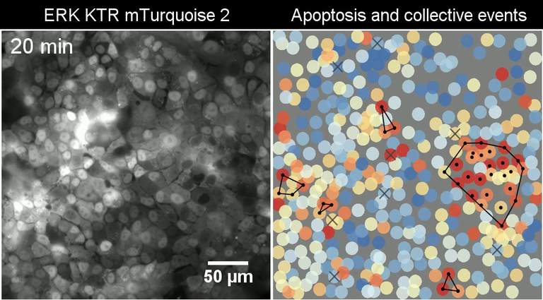
Collective ERK activation due to apoptosis in MCF10A WT cells

Despite its focus on cell signalling, the framework can be also applied to other spatially correlated phenomena that occur over time in an arbitrary spatial dimension.

Implementations

This repository covers the R implementation. For other implementations check:

arcos4py, a Python implementation written by Benjamin Grädel.
arcos-gui, a plugin with GUI for napari image viewer; written by Benjamin Grädel. See a YouTube demo.

Documentation for the entire ARCOS project can be found on gitbook.

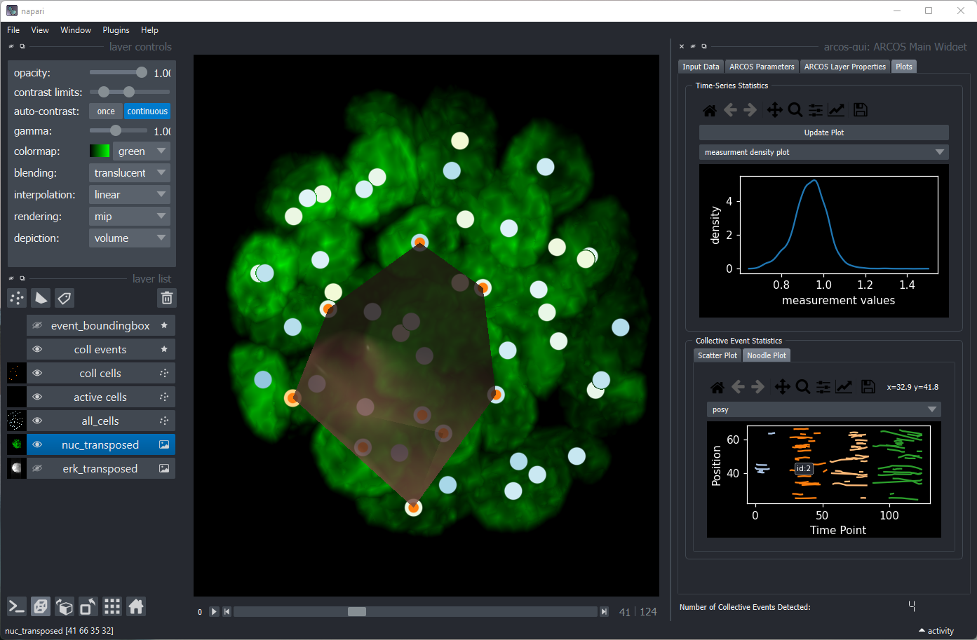
arcos-gui plugin for napari image viewer

Installation

You can install the development version from GitHub with:

# install.packages("devtools")
devtools::install_github("dmattek/ARCOS")

The algorithm

The algorithm implemented in the ARCOS::trackColl function consists of two steps:

In every frame, objects are clustered with the dbscan algorithm.
Clusters are linked between the frames if objects that comprise the cluster are within a threshold distance.

The RANN::nn2 function is used to calculate nearest neighbour distances. The dbscan::dbscan function is used for spatial clustering.

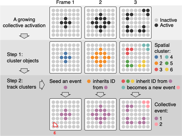
ARCOS algorithm on a single event

The flowchart of the algorithm:

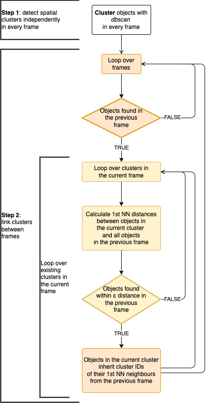
ARCOS algorithm flowchart

Functions

Main functions:

arcosTS creates an arcosTS object from time series data in long format stored in a data.table. Assigns relevant column names and data parameters.
trackColl identifies and tracks collective events.

Visualisation functions:

plotTracks plots a random selection of tracks in 1 or 2D.
plotNoodle2D creates a noodle/spaghetti plot; a single position coordinate is plotted over time for objects during their participation in collective events.
runCollVis visualises collective events in an interactive shiny app.

Post-processing:

calcNNdists calculates nearest neighbour distances between objects to give an idea about the search radius for spatial clustering.
calcStatsColl calculates basic statistics of collective events such as duration and size.
selColl selects collective events based on their duration and size.

Export functions:

export2napari exports data as several files that can be imported as layers into napari image viewer.
savePlotColl2D saves individual frames as images.

Measurement pre-processing:

interpolMeas interpolates missing data in time series.
histMeas plots a histogram of the measurement.
clipMeas clips the measurement to a prescribed range or quantiles.
binMeas de-trends, normalises and binarises the measurement in time series.
plotBinMeas plots sample time series and visualises measurement de-trending/rescaling/binarisation.
histTrackLen plots a histogram of track lengths.
selTrackLen selects tracks from time series data based on their length.

Utility functions:

is.arcosTS checks whether an object is an arcosTS object.
keepSignifDig trims numeric columns to a prescribed number of significant digits.
genSynth2D generate synthetic data in 2D with a single collective event over 8 frames.
genRandSynth2D generate a random sequence of synthetic collective events in 2D.
loadDataFromFile loads time series data from a file and returns an arcosTS object.
loadDataFromImages loads time series data from images and returns an arcosTS object.

1D example

Here, 4 distinct objects are moving in 1 dimension over 5 time points. We aim to identify clusters of objects moving close to each other.

Time sequence

The minimal data in long format consists of 3 columns:

frame with the frame number that corresponds to the time point,
objid with the unique identifier of every object,
x with the position of the object.

dts1 = data.table(frame = c(1, 1, 2, 2, 2, 3, 3, 3, 3, 4, 4, 4, 5, 5),
                  objid = c(1, 2, 1, 2, 3, 1, 2, 3, 4, 1, 2, 4, 1, 4),
                  x = c(1, 3, 1.2, 2.5, 3.5, 0.9, 2.6, 2.9, 3.2, 1.1, 2.8, 3.1, 1, 3))

knitr::kable(dts1)

frame	objid	x
1	1	1.0
1	2	3.0
2	1	1.2
2	2	2.5
2	3	3.5
3	1	0.9
3	2	2.6
3	3	2.9
3	4	3.2
4	1	1.1
4	2	2.8
4	4	3.1
5	1	1.0
5	4	3.0

Initiate an arcosTS object. Specify the names of frame, object id, and positions columns. The function simply adds attributes to the existing data.table object.

ARCOS::arcosTS(dt = dts1, 
               colFrame = "frame", 
               colIDobj = "objid", 
               colPos = "x")

Plot the time series. Each object has a distinct identifier represented by a different colour in the plot:

ARCOS::plotTracks(dts1)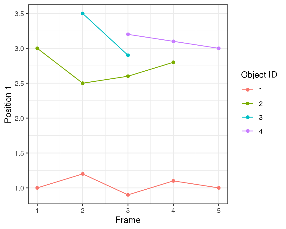

Detection and tracking

In this step 3 objects at the top are grouped into a single collective event that spans 5 frames. A single object at the bottom forms a single-object event.

The most important parameter of the trackColl function is the search radius eps, which sets the distance for:

the dbscan spatial clustering in a single time frame,
linking clusters between frames; clusters in consecutive frames are linked, if objects comprising them are within the threshold radius.

The minimum size of the spatial cluster is set using the minClSz parameter, which is also passed to dbscan. The parameter nPrev determines the number of previous frames that are searched for collective events in order to link them to the current frame.

dcoll1 = ARCOS::trackColl(dts1)

The output contains 3 columns with the frame number, object identifier, and the calculated identifier of the collective event:

frame	objid	collid.frame	collid	x
1	1	1	1	1.0
1	2	2	2	3.0
2	1	3	1	1.2
2	2	4	2	2.5
2	3	4	2	3.5
3	1	5	1	0.9
3	2	6	2	2.6
3	3	6	2	2.9
3	4	6	2	3.2
4	1	7	1	1.1
4	2	8	2	2.8
4	4	8	2	3.1
5	1	9	1	1.0
5	4	10	2	3.0

Visualisation

Each trace is assigned an identifier of the collective event, which is represented by the shape of the point in the plot:

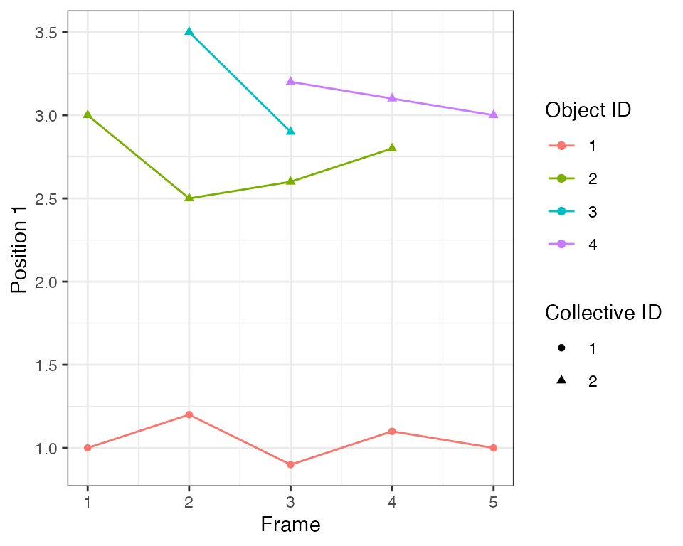
The algorithm with the default search radius eps=1.0 has identified two collective events. One is an event with only a single object, the latter is an event that consists of 1 to 3 objects at different points in time.

2D example

The following synthetic dataset contains 81 objects (e.g., biological cells) spaced on a 2D 9x9 lattice with a spacing of 1x1 length units. Each object has an ID (column id) and can assume values 0 and 1 (column m), which correspond to an inactive and active state. The evolution of active states takes place over 8 consecutive time points (column t). Each object wiggles slightly around its position.

# Generate a synthetic dataset with a single event evolving over 8 frames
dts2 = ARCOS::genSynthSingle2D(inSeed = 7)

knitr::kable(head(dts2), digits = 2)

t	x	y	id
1	0.23	-0.16	1
1	0.88	-0.12	2
1	1.93	0.08	3
1	2.96	0.19	4
1	3.90	-0.04	5
1	4.91	0.07	6

In the plot below, grey circles correspond to inactive and black to active states of cells and their collective activation (wave) develops over 8 time points.

p1 = ggplot(dts2,
            aes(x = x,
                y = y)) +
  geom_point(aes(color = as.factor(m)), size = 5) +
  scale_color_manual(values = c("grey80",
                                "grey20")) +
  facet_wrap(~ t, ncol = 4) +
  coord_fixed(ratio=1) +
  theme_void() +
  theme(text = element_text(size = 20),
        legend.position = "none")

p1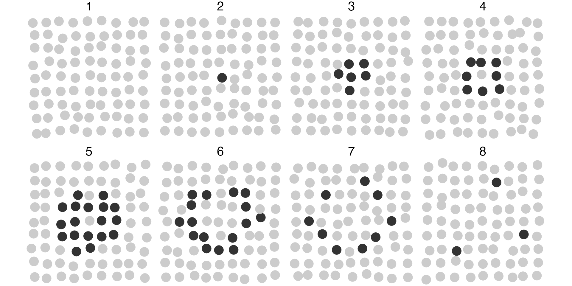

Identify collective events

The following R code will identify the collective event and store the result in a dcoll variable. We are interested in a collective event comprised of active objects, hence we select rows with m > 0. The parameter eps sets the threshold radius for the spatial clustering (dbscan algorithm). Here, we set eps = 2, which is enough to find all the nearest active objects in the cluster, given the 1x1 horizontal and vertical spacing of objects in the lattice.

# Track collective events
dcoll2 = ARCOS::trackColl(dts2[m > 0], 
                          eps = 2.)

knitr::kable(head(dcoll2), digits = 2)

t	id	collid.frame	collid	x	y	m
2	41	1	1	4.16	3.91	1
3	32	2	1	3.89	2.99	1
3	40	2	1	3.09	4.19	1
3	41	2	1	4.00	3.96	1
3	42	2	1	5.06	4.06	1
3	50	2	1	3.84	4.91	1

The dcoll table contains the results of spatio-temporal clustering. Column collid stores a unique identifier of collective event. The collid.frame column stores an identifier of collective event that is unique only within a frame.

Visualise events

For better visualisation, we add convex hulls around collective events using the chull function from the grDevices package.

# Create convex hulls around collective events fro visualisation
dcollch2 = dcoll2[,
                  .SD[grDevices::chull(x, y)],
                  by = .(t,
                         collid)]

In the following plot, objects that participate in collective events are indicated by red dots. The red polygon indicates a convex hull.

p2 = ggplot(dts2,
            aes(x = x,
                y = y)) +
  geom_point(aes(color = as.factor(m)), size = 5) +
  scale_color_manual(values = c("grey80",
                                "grey20")) +
  ggnewscale::new_scale_color() +
  geom_point(data = dcoll2,
             aes(color = as.factor(collid)), size = 1) +
  geom_polygon(data = dcollch2,
               aes(color = as.factor(collid)),
               fill = NA, 
               size = 1) +
  facet_wrap(~ t, ncol = 4) +
  coord_fixed(ratio=1) +
  theme_void() +
  theme(text = element_text(size = 20),
        legend.position = "none")
#> Warning: Using `size` aesthetic for lines was deprecated in ggplot2 3.4.0.
#> ℹ Please use `linewidth` instead.

p2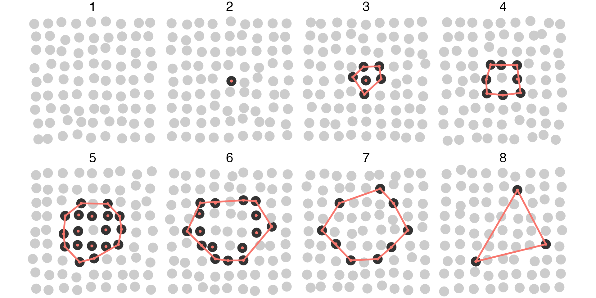

Spaghetti/noodle plot

Spaghetti/noodle plot is another useful visualisation of collective events. A single position of cell tracks is plotted over time, however cells tracks are plotted only when objects/cells participate in the collective event.

ARCOS::plotNoodle2D(dcoll2, style = 'both') +
  xlab("Time [frames]") +
  ylab("Position X [au]") +
  theme_minimal() +
  theme(legend.position = "none")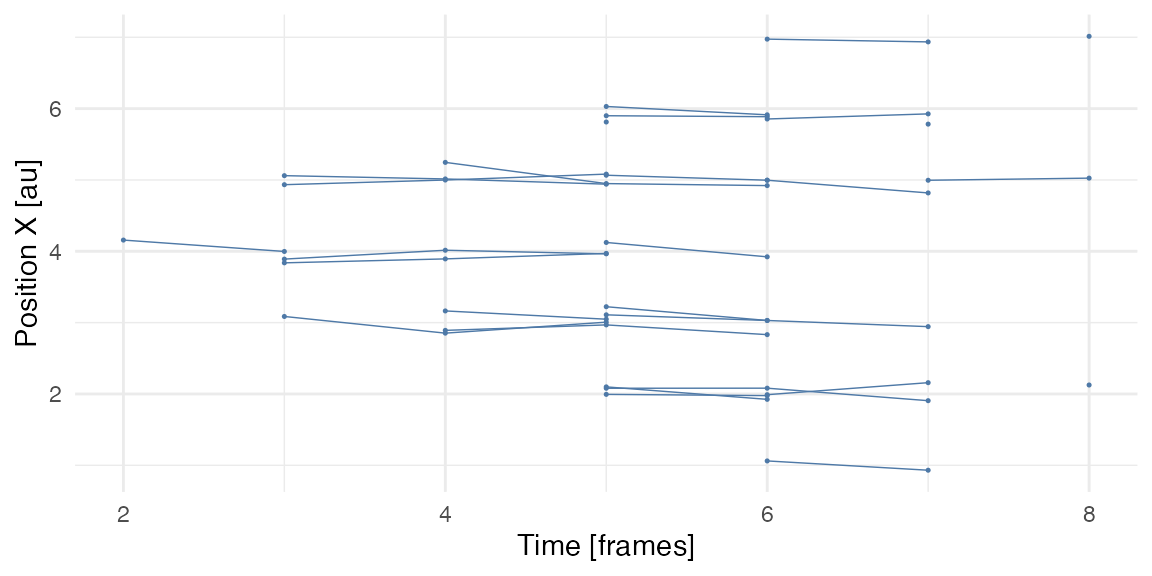

Extract measurements

Growth over time

dcoll2growth = calcGrowthColl(dcoll2)

ggplot(dcoll2growth,
       aes(x = tevent,
           y = diam)) +
  geom_line() +
  geom_point() +
  xlab("Time of the event [frames]") +
  ylab("Diameter [au]") +
  theme_bw()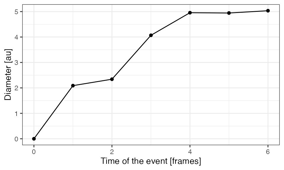

### Size & duration

Extract duration (totDur), total number of unique objects involved in the event (totSz), the smallest and largest number of objects in the event (minSz & maxSz).

knitr::kable(calcStatsColl(dcoll2))

collid	clDur	minSz	maxSz	totSz
1	7	1	18	27

Save frames

The code below saves individual time frames with the field of view as png files in the frames folder located in the current working directory.

ARCOS::savePlotColl2D(dts2, dcoll2, 
                      outdir = "./frames",
                      xlim = c(-.5,9),
                      ylim = c(-.5,9),
                      plotwh = c(4,3),
                      imtype = "png")

Individual files can be later combined into a movie using software such as ffmpeg.

For example, if you have ffmpeg installed on your system, create an mp4 movie at 2 frames/second and a 520x420 pixel resolution by typing the following line in the command line:

ffmpeg -framerate 2 -i "frames/F%04d.png" -vcodec libx264 -s 560x420 -pix_fmt yuv420p frames-all.mp4

Visualise interactively

Interactive visualisation with an accompanying shiny app located in inst/shiny-examples/collVisApp.

library(shiny)
library(plotly)
library(RColorBrewer)

ARCOS::runCollVis(dts2, dcoll2)

frame	objid	x
1	1	1.0
1	2	3.0
2	1	1.2
2	2	2.5
2	3	3.5
3	1	0.9
3	2	2.6
3	3	2.9
3	4	3.2
4	1	1.1
4	2	2.8
4	4	3.1
5	1	1.0
5	4	3.0

frame	objid	collid.frame	collid	x
1	1	1	1	1.0
1	2	2	2	3.0
2	1	3	1	1.2
2	2	4	2	2.5
2	3	4	2	3.5
3	1	5	1	0.9
3	2	6	2	2.6
3	3	6	2	2.9
3	4	6	2	3.2
4	1	7	1	1.1
4	2	8	2	2.8
4	4	8	2	3.1
5	1	9	1	1.0
5	4	10	2	3.0

frame	objid	x
1	1	1.0
1	2	3.0
2	1	1.2
2	2	2.5
2	3	3.5
3	1	0.9
3	2	2.6
3	3	2.9
3	4	3.2
4	1	1.1
4	2	2.8
4	4	3.1
5	1	1.0
5	4	3.0

frame	objid	collid.frame	collid	x
1	1	1	1	1.0
1	2	2	2	3.0
2	1	3	1	1.2
2	2	4	2	2.5
2	3	4	2	3.5
3	1	5	1	0.9
3	2	6	2	2.6
3	3	6	2	2.9
3	4	6	2	3.2
4	1	7	1	1.1
4	2	8	2	2.8
4	4	8	2	3.1
5	1	9	1	1.0
5	4	10	2	3.0

frame	objid	x
1	1	1.0
1	2	3.0
2	1	1.2
2	2	2.5
2	3	3.5
3	1	0.9
3	2	2.6
3	3	2.9
3	4	3.2
4	1	1.1
4	2	2.8
4	4	3.1
5	1	1.0
5	4	3.0

frame	objid	collid.frame	collid	x
1	1	1	1	1.0
1	2	2	2	3.0
2	1	3	1	1.2
2	2	4	2	2.5
2	3	4	2	3.5
3	1	5	1	0.9
3	2	6	2	2.6
3	3	6	2	2.9
3	4	6	2	3.2
4	1	7	1	1.1
4	2	8	2	2.8
4	4	8	2	3.1
5	1	9	1	1.0
5	4	10	2	3.0