Pre-processing time-series for ARCOS
Source:vignettes/ARCOS-binTimeseries.Rmd
ARCOS-binTimeseries.RmdIntro
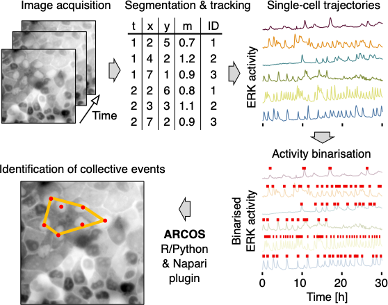
Using ARCOS to detect collective activation events in biological systems requires identification of active objects, i.e., objects that will be passed to the clustering algorithm. In practice the single-cell activity obtained from image segmentation needs to be thresholded and binarised. ARCOS offers several approaches to perform such approaches that will be covered below.
The pipeline
Load time-series data
Time-series data obtained, for example, from image segmentation should be in long format. Here we use a sample dataset of single-cell ERK activity from MCF10A WT epithelial cells. See the associated publication on bioRxiv for more details about biological problems that can be analysed with ARCOS.
# define column names
lCols = list()
lCols$frame = 'frame'
lCols$trackid = 'trackid'
lCols$posx = 'x'
lCols$posy = 'y'
lCols$meas = 'meas'

# Load from file
dts = fread(system.file('testdata/sampleTS.csv.gz',
                        package = 'ARCOS'))

# create an ARCOS ts object
ARCOS::arcosTS(dts,
               colPos = c(lCols$posx, lCols$posy),
               colMeas = lCols$meas,
               colFrame = lCols$frame,
               colIDobj = lCols$trackid)

knitr::kable(head(dts, 4), digits = 2)| frame | trackid | x | y | meas |
|---|---|---|---|---|
| 0 | 16 | 682.21 | 148.14 | 0.49 |
| 1 | 16 | 679.79 | 149.04 | 0.48 |
| 2 | 16 | 678.68 | 149.87 | 0.48 |
| 3 | 16 | 680.24 | 148.45 | 0.48 |
Measurement interpolation
The measurement may contain missing values or NAs, which can be
interpolated using the ARCOS::interpolMeas function.
# interpolate
dts = ARCOS::interpolMeas(dts)
#> Registered S3 method overwritten by 'quantmod':
#>   method            from
#>   as.zoo.data.frame zoo
Measurement distribution
Point outliers in the measurement can be clipped using the
ARCOS::clipMeas function.
ARCOS::histMeas(dts,
                clip = c(0.001, 0.999),
                quant = TRUE) +
  ggthemes::theme_clean()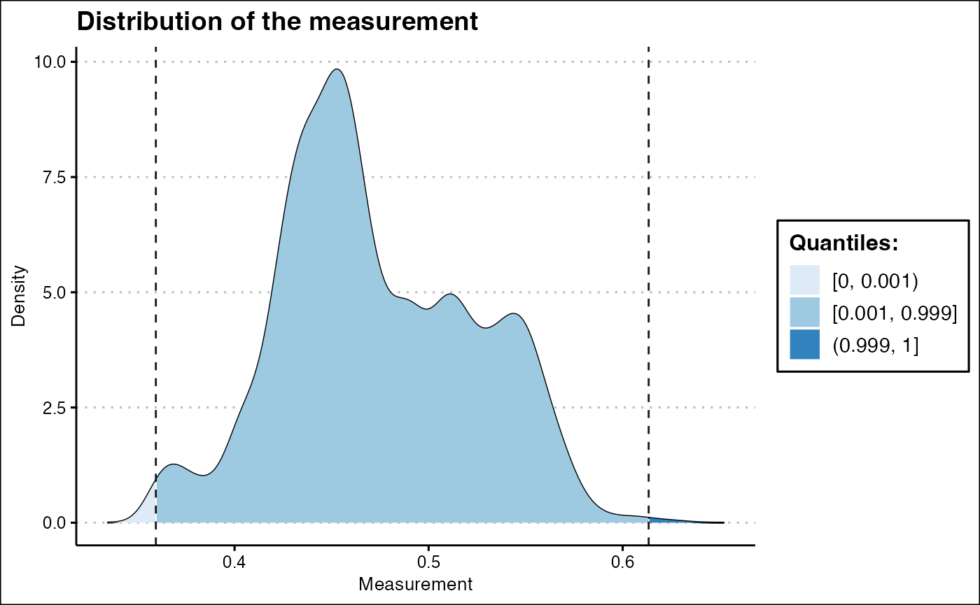
Track lengths
De-trending is based on a running median, therefore, it requires time series that are approximately at least 4 times longer than the length of the de-trending median filter.
ARCOS::histTrackLen(dts, binwidth = 10) 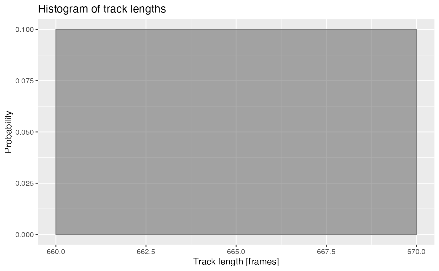
Length of time series in frames. Frames acquired every 1 minute.
dts = ARCOS::selTrackLen(dts, lenmin = 660)

knitr::kable(
  dts[,
      .N,
by = trackid])| trackid | N |
|---|---|
| 16 | 661 |
| 20 | 661 |
| 22 | 661 |
| 74 | 661 |
| 107 | 661 |
| 108 | 661 |
| 118 | 661 |
| 131 | 661 |
| 230 | 661 |
Identify activity
Regions of measurement activity identified with several methods
available in the ARCOS::binMeas function.
runmed
This approach uses a short-term smoothing filter to remove noise from time series and a long-term filter to remove trends.
- Short-term smoothing to filter noise (median filter with \(k = 5\) frames).
- Long-term smoothing to de-trend (median filter with \(k = 201\) frames).
- Rescale if the difference between min and max is greater than \(peakThr = 0.05\).
- Binarise the final signal with \(binThr = 0.1\).
# binarise the measurement
ARCOS::binMeas(dts,
               biasMet = "runmed",
               smoothK = 5L,
               biasK = 501L,
               peakThr = 0.05,
               binThr = 0.1)
The ARCOS::binMeas function adds meas.resc
and meas.bin columns to the original dataset. Below is the
plot of original time series compared to de-trended/rescaled and
binarised output. The meas.bin column should be used to
filter the rows such that only active cells are used to detect
collective events, i.e.,
ARCOS::trackColl(dts[meas.bin > 0]).
| frame | trackid | x | y | meas | meas.resc | meas.bin |
|---|---|---|---|---|---|---|
| 0 | 16 | 682.21 | 148.14 | 0.49 | 0 | 0 |
| 1 | 16 | 679.79 | 149.04 | 0.48 | 0 | 0 |
| 2 | 16 | 678.68 | 149.87 | 0.48 | 0 | 0 |
| 3 | 16 | 680.24 | 148.45 | 0.48 | 0 | 0 |
| 4 | 16 | 679.30 | 149.14 | 0.47 | 0 | 0 |
| 5 | 16 | 678.61 | 148.03 | 0.47 | 0 | 0 |
p1 = ARCOS::plotBinMeas(dts,
                        ntraj = 0L,
                        xfac = 1 / 60.,
                        plotResc = TRUE,
                        inSeed = 3L) +
  geom_hline(yintercept = 0.1,
             color = "#F28E2B",
             linetype = "dashed") +
  ggthemes::theme_few() +
  xlab("Time [h]") +
  ylab("C/N ERK-KTR")

p1
#> Warning: Removed 304 rows containing missing values (`geom_path()`).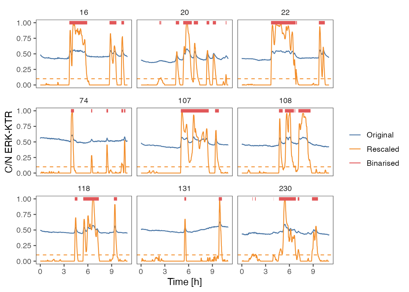
lm
In this approach, a fit to a linear function is used to de-trend the time series.
- Short-term smoothing to filter noise (median filter with \(k = 5\)).
- De-trend by fitting a 5th order polynomial (median filter with \(polyDeg = 5\)).
- Rescale if the difference between min and max is greater than \(peakThr = 0.2\).
- Binarise the final signal with \(binThr = 0.2\).
# binarise the measurement
ARCOS::binMeas(dts,
               biasMet = "lm",
               smoothK = 5L,
               peakThr = 0.05,
               polyDeg = 5L,
               binThr = 0.2)

ARCOS::plotBinMeas(dts,
                   ntraj = 0L,
                   xfac = 1 / 60.,
                   plotResc = TRUE,
                   inSeed = 3L) +
  geom_hline(yintercept = 0.2,
             color = "#F28E2B",
             linetype = "dashed") +
  ggthemes::theme_few() +
  xlab("Time [h]") +
  ylab("C/(C+N) ERK-KTR")
#> Warning: Removed 131 rows containing missing values (`geom_path()`).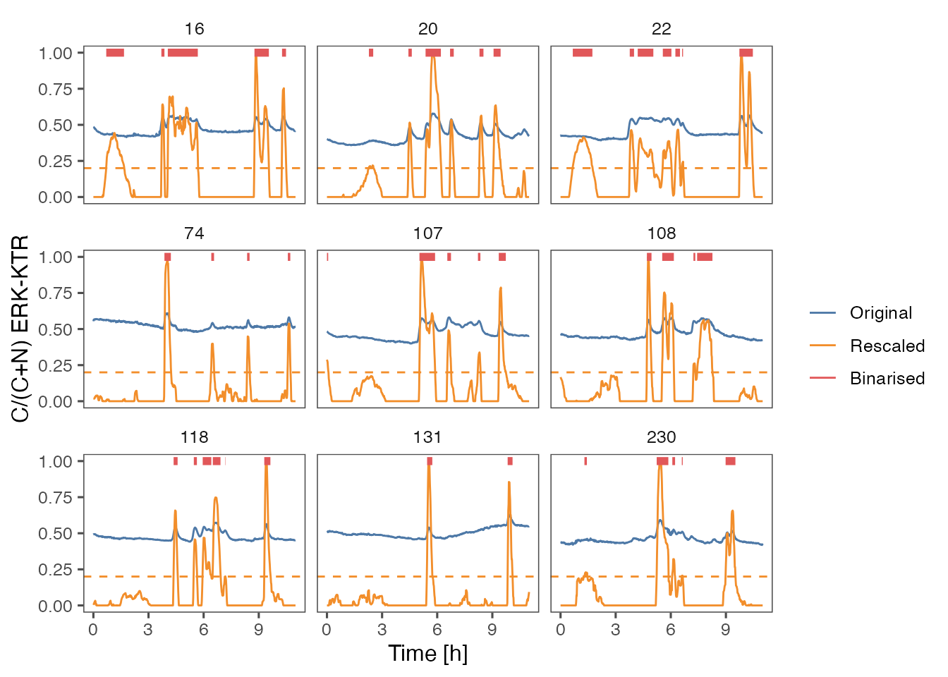
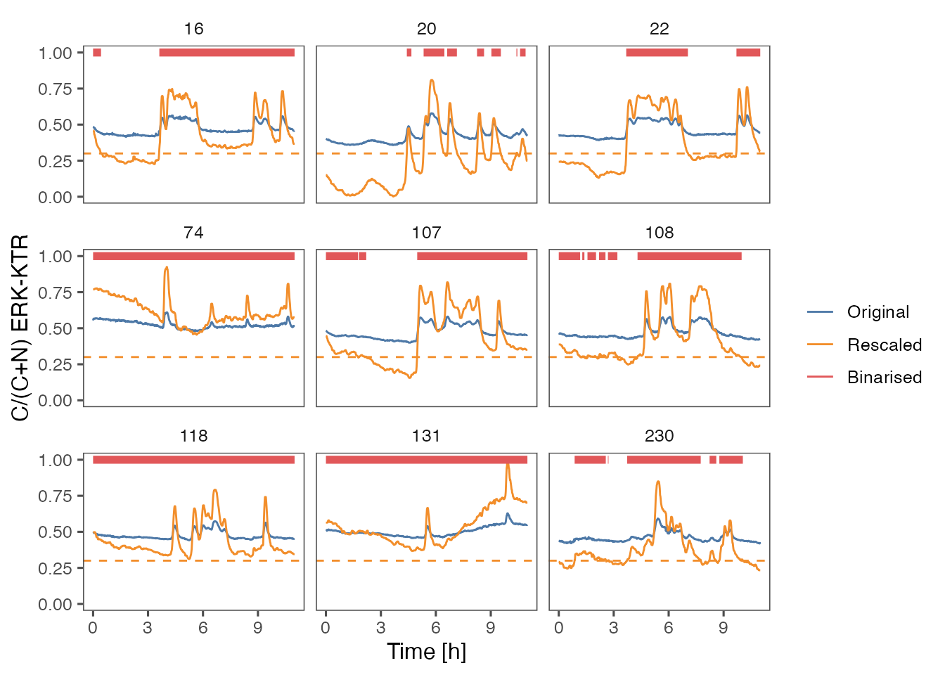
none
In this approach a fixed threshold is applied to rescaled time series.
- Rescale all time series between global min and max.
- Short-term smoothing to filter noise (median filter with \(k = 5\)).
- Binarise the final signal with \(binThr = 0.3\).
# binarise the measurement
ARCOS::binMeas(dts,
               biasMet = "none",
               smoothK = 5L,
               binThr = 0.3)

ARCOS::plotBinMeas(dts,
                   ntraj = 0L,
                   xfac = 1 / 60.,
                   plotResc = TRUE,
                   inSeed = 3L) +
  geom_hline(yintercept = 0.3,
             color = "#F28E2B",
             linetype = "dashed") +
  ggthemes::theme_few() +
  xlab("Time [h]") +
  ylab("C/(C+N) ERK-KTR")
#> Warning: Removed 57 rows containing missing values (`geom_path()`).